In image processing, two concepts are of fundamental importance: Gaussian noise and Gaussian Filter. A solid understanding of these two concepts will pave a smooth path for further studies.

We can conveniently think of noise as the unwanted signal in an image. Noise is random in nature. Gaussian noise is a type of noise that follows a Gaussian distribution.

A fitler is a tool. It transforms images in various ways. A Gaussian filter is a tool for de-noising, smoothing and blurring.

Why is Gaussian noise important in image processing?

Noise in images arises from various sources. Under most conditions, these noises follow a Gaussian distribution and therefore are refered to as Gaussian noises. The main source of Gaussian noise includes sensor noise and electronic circuit noise.

There are also noises that follow other probability distributions, e.g. shot noise can be described by a poisson distribution. However, according to the central limit theorem, when random variables that follow different distribuions are added together, the sum tends to follow a Gaussian distrbution. Therefore, when we develop a single-noise model, as will be described next, we often choose to describe the noise as Gaussian.

A Gaussian noise model for images

When we talk about the Gaussian noise in an image, usually we are thinking of additive Gaussian noise. In other words, if we describes the uncontaminated, free-of-noise source image as \(S(x,y)\), then the observed image \(O(x,y)\) is given by:

\[O(x,y) = S(x,y) + e(x,y)\]

where each \(e(x,y)\) is drawn from a Gaussian distribution. If we assume the noise is white, as we usually do, then each pair of \(e(x_1,y_1)\) and \(e(x_2,y_2)\) are independent of each other. Another assumption is every \(e(x,y)\) is drawn from the same Gaussian distrubtion. In short, we say \(e(x,y)\) is independently and identically distributed (often abbreviated as iid).

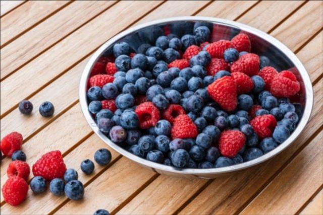
It is easy to simulate such noise in an image. Shown below are the source image and its Gaussian-noise-contaminated versions, and the python code that generated these images.

import numpy as np

import matplotlib.pyplot as plt
import matplotlib.image as mpimg

img=mpimg.imread('berries.jpg')
plt.figure(0)
imgplot = plt.imshow(img)

height = img.shape[0]
width = img.shape[1]

#Create an array of noise by drawing from a Gaussian distribution
#Add to source image
#Clip at [0, 255]
n_20 = np.random.normal(0, 20, [height, width, 3])
noisy_20_img = (img+n_20).clip(0,255)

n_50 = np.random.normal(0, 50, [height, width, 3])
noisy_50_img = (img+n_50).clip(0,255)

plt.figure(1)
imgplot = plt.imshow(noisy_20_img.astype('uint8'))

plt.figure(2)
imgplot = plt.imshow(noisy_50_img.astype('uint8'))

Gaussian filter

A filter is defined by its kernel. When we apply a filter to an image, the result is the convolution between the kernel and the original image.

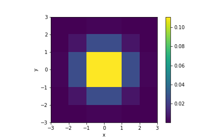
The kernel of a Gaussian filter is a 2d Gaussian function (Fig.2). When such a kernel is convolved with an image, it creates a blurring effect. This is because each pixel is now assigned with a weighted sum of itself and its neighbouring pixels. Any discontinuities in the neighbourhood are thereby averaged out.

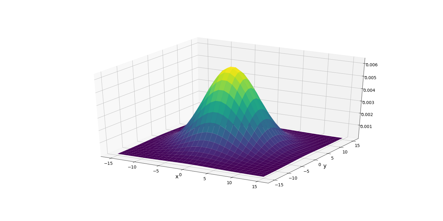
A 2d Gaussian function is defined over the entire real plane while, surely, a Gaussian kernel must be of a finite size. Therefore we must truncate the Gaussian function at some threshold. A resonable choice would be 3 times the function's standard deviation (\(\sigma\)). This is equivalent to saying that, during convolution, pixels that are at a distance more than 3\(\sigma\) away do not contribute to the current pixel's new value.

Shown below are several Gaussian kernels, each has a different \(\sigma\), but all truncated at 3\(\sigma\), and the blurred images they produced.

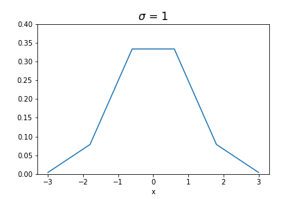
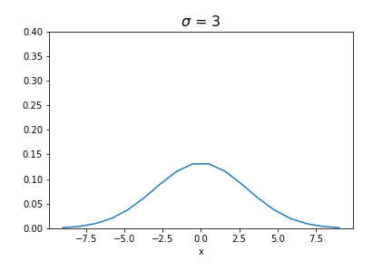
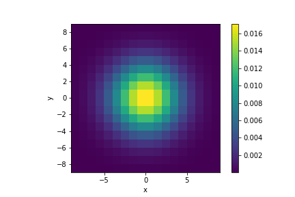
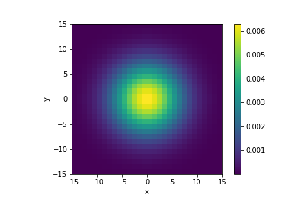
It can be seen that as the kernel size grows larger, the blurring effect becomes more prominent. The code for applying the Gaussian kernel to create the blurred image is shown below:

import math
from scipy import signal

import matplotlib.pyplot as plt

#standard deviation
sigma = 5
N = 6*sigma

# create a Gaussian function truncated at [-3*sigma, 3*sigma]
t = np.linspace(-3*sigma, 3*sigma, N)
gau = (1/(math.sqrt(2*math.pi)*sigma))*np.exp(-0.5*(t/sigma)**2)

# create a 2d Gaussian kernel from the 1d function
kernel = gau[:,np.newaxis]*gau[np.newaxis,:]

# convolve the image with the kernel
blurred = signal.fftconvolve(img, kernel[:, :, np.newaxis], mode='same')

# rescale to [0, 255]
blurred = (blurred - blurred.min())/(blurred.max()- blurred.min())*255

plt.imshow(blurred.astype('uint8'))

Is Gaussian filter good for eliminating Gaussian noise?

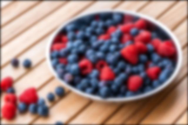
The short answer is no. Although they share the same name, one is not the remedy of the other, or at least not an optimal one. As shown in the pictures below, while a sufficienly large kernel can remove most of the Gaussian noise, it also takes away a lot of details of the image. To preserve the details while de-noising, one should consider the edge-preserving filters, such as the median filter and the bilateral filter.